Voxel Data Storage
Data storage is the second challenge to overcome. If the game has a reasonable, fixed size, and you can afford to store all data at once, you might as well just store it in a large 3D array. Geometrically, each element in the 3 dimensional array represents a 1x1x1 area.

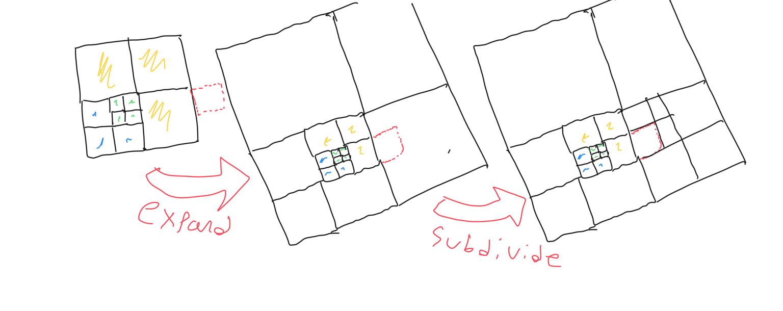
More often, though, you’ll either want the map size to be infinite or at least large enough that you can’t store all of that information at once. For that, you’ll need to break the map apart into reasonably sized pieces that can be read from and written to memory. There is often a bit of nuance with regards to threading and ensuring that you only attempt to generate mesh for a chunk when its neighbors are loaded too. There is always mesh data along the edge of each chunk that cannot be generated without data from other chunks. This is sometimes referred to as the skirt, which usually has some unique considerations, especially when threading is involved. Each element in each 3 dimensional array is still responsible for a 1x1x1 volume, but additionally, each chunk is responsible for a larger defined volume as well.
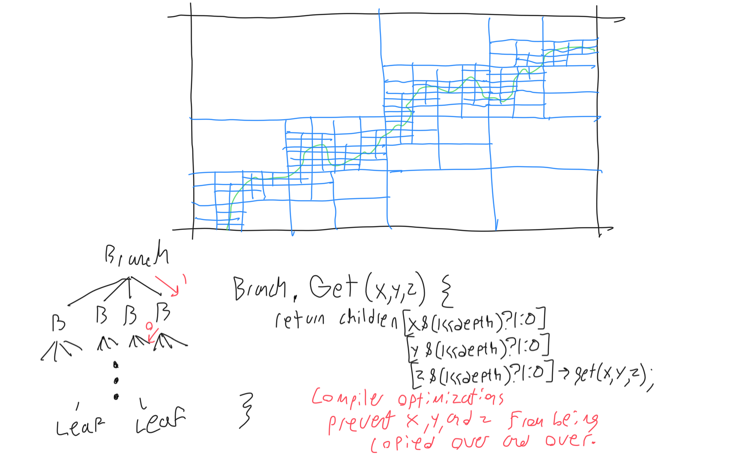
For very fine voxel resolutions, you’ll want to construct an octree. An octree is a recursive structure where 3D space is recursively subdivided into 8 regions. Any area that is one solid type of voxel does not need to be subdivided and is stored as one id. As you can see in the figure, for finer resolutions, there is a significant reduction in memory usage. The octree offers this reduction because volumetric data often has large, contiguous, homogenous areas. Now that our volumetric data is stored as a tree, we should access it similarly to doing a binary search. The figure below provides a visual explanation of why we can use the binary representation of the block’s coordinates to get its place in the tree. Reading from and writing to a file is still trivial- the octree must be saved recursively. The octree has restrictions on it that allow it to function. The octree always has a ‘bottom’, where it will not divide area any further. Branches must know how far they are above this bottom- this will determine if they are accountable for a 2x2x2 volume, a 4x4x4 volume, an 8x8x8 volume, etc. Branches will always be accountable for cubic volume whose side lengths are a power of two above one. Solid areas that are not subdivided are stored as buds, which are the same but there can be 1x1x1 sized buds. (Other tree structures for storing different kinds of data will always be size 1x1x1).
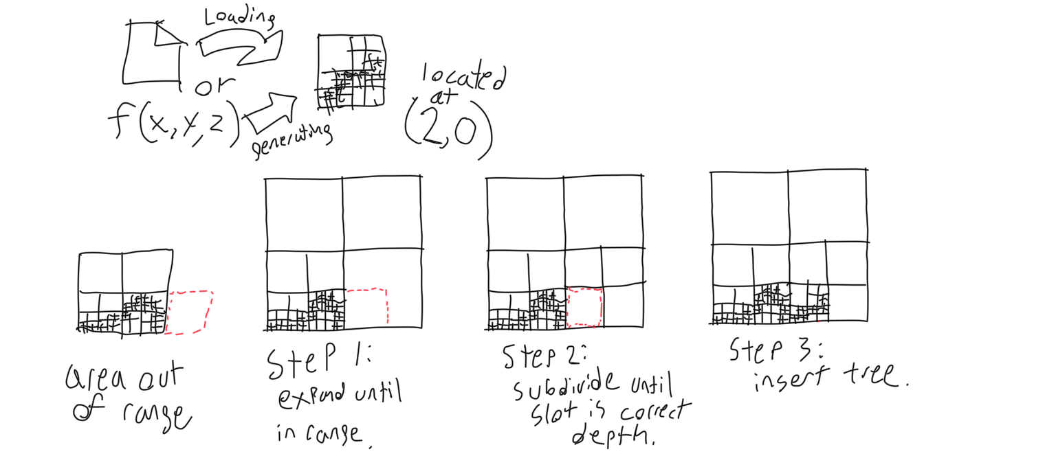
In order to use an octree with an infinite world size, the last two methods can be combined- data is loaded and unloaded in portions with an octree representation. Instead of having an octree for each chunk, though, it’s faster to combine all of the octrees into one octree that expands as more data is loaded in. Without negative values, it’s easy to see how this would work. The tree representing some chunk is loaded, and then must be inserted into the world tree. First, the world tree must grow large enough to encapsulate the area inhabited by the chunk. Growing an octree is done by creating a new root node whose children consist of seven buds and the previous root node. The previous root node will be the lower left child, which ensures that the octree will expand up and to the right. The new root node will be twice as large in each dimension. Then, the tree must recursively divide the appropriate bud until there is a spot for the chunk to be placed. To divide a bud, the bud is replaced with a branch of the same size whose children are smaller buds. Only then can the chunk be placed in the world tree.
To allow for negative values, a change must be made to the octree. When the tree expands, it has to expand in the negative direction as well as the positive direction. To accomplish this, the octree will alternate between making the old root node the new root node’s lower left child and making it the new root node’s upper right child. Geometrically speaking, the octree alternates between doubling forward and doubling backward. This is an extremely effective method for encapsulating all of space, but it makes finding locations in the tree more difficult.
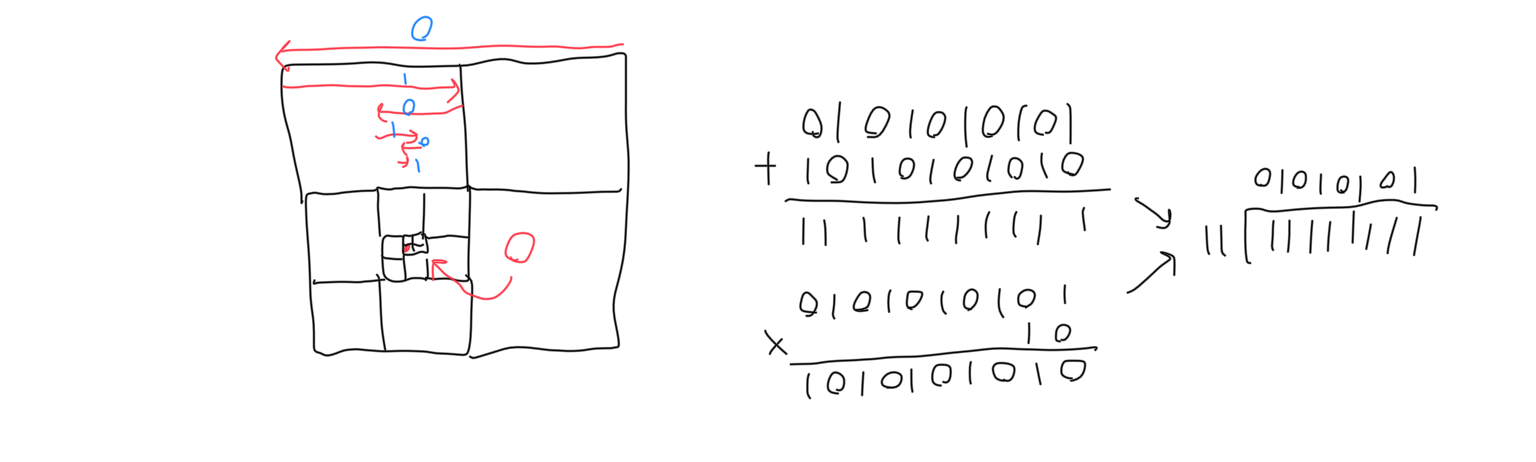
A voxel’s location in the tree is no longer the same as its binary representation. Relying on the binary representation of the number to ‘wrap around’ would be unacceptable because it would cause discontinuities once the tree expands and begins taking the next most significant bit into consideration. The coordinates of each voxel must be transformed into ‘address space’ before their binary representations may be used to find its position in the tree. This transformation can be observed to be associative with addition (voxels have different addresses but consecutive addresses are still consecutive), which means to transform into address space is to add a certain offset to the coordinate and then take the binary representation. That offset should be 0 in address space, which logically I know has to be the repeating binary pattern 10101010.... Because the tree alternates between expanding positively and negatively, alternating between going down the left side of the tree and the right side will eventually end up at zero. I use a slight modification to this that ensures that chunk coordinates can be found by truncated division by the chunk size.
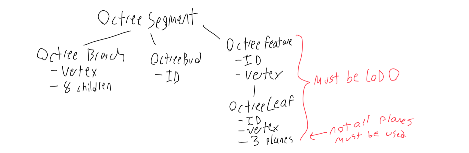
The tree can also be used to store hermitian data, but some small changes should be made. In addition to branches, for areas that contain changes, and buds, for uniform areas, There should also be features for areas that need to store a vertex and leaves for areas that need to store edges. As opposed to branches and buds, features and leaves are always size 1x1x1. The following diagram shows the inheritance tree or these structures.