Voxel Data Visualization
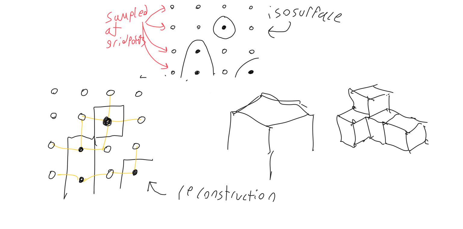
The first thing needed for a voxel engine is called an isosurface. An isosurface is a multidimensional function where negative values are intended to be outside the ‘solid’ and positive values are intended to be inside the solid. Interesting ones that resemble roads, mountains, and valleys can come later, but right now simple isosurfaces like spheres and planes are useful for testing. Isosurfaces are only used to generate the initial terrain- once generated, the terrain can be changed to no longer resemble the function. Isosurface functions only need to be fast to execute- they need not have a known derivative, integral, or any other property. Rather, they are sampled. The function is called at every 3d gridpoint in the game world, with the assumption that for each two points, if one is positive and the other negative, the solid has boundary that exists between those so points. Isosurfaces are useful for the voxel engine because they are very flexible, so most generation is done using them.

The second thing needed for a voxel engine is a method to turn volumetric data into a visible mesh. The simplest way to do this is intuitive: create a square on each boundary between transparent and opaque material. The isosurface must be sampled at each 3d gridpoint, and then this data must be remembered. This is the method most are familiar with, thanks to Minecraft. This is a very fast approach that makes texturing easy, but the results are always blocky.
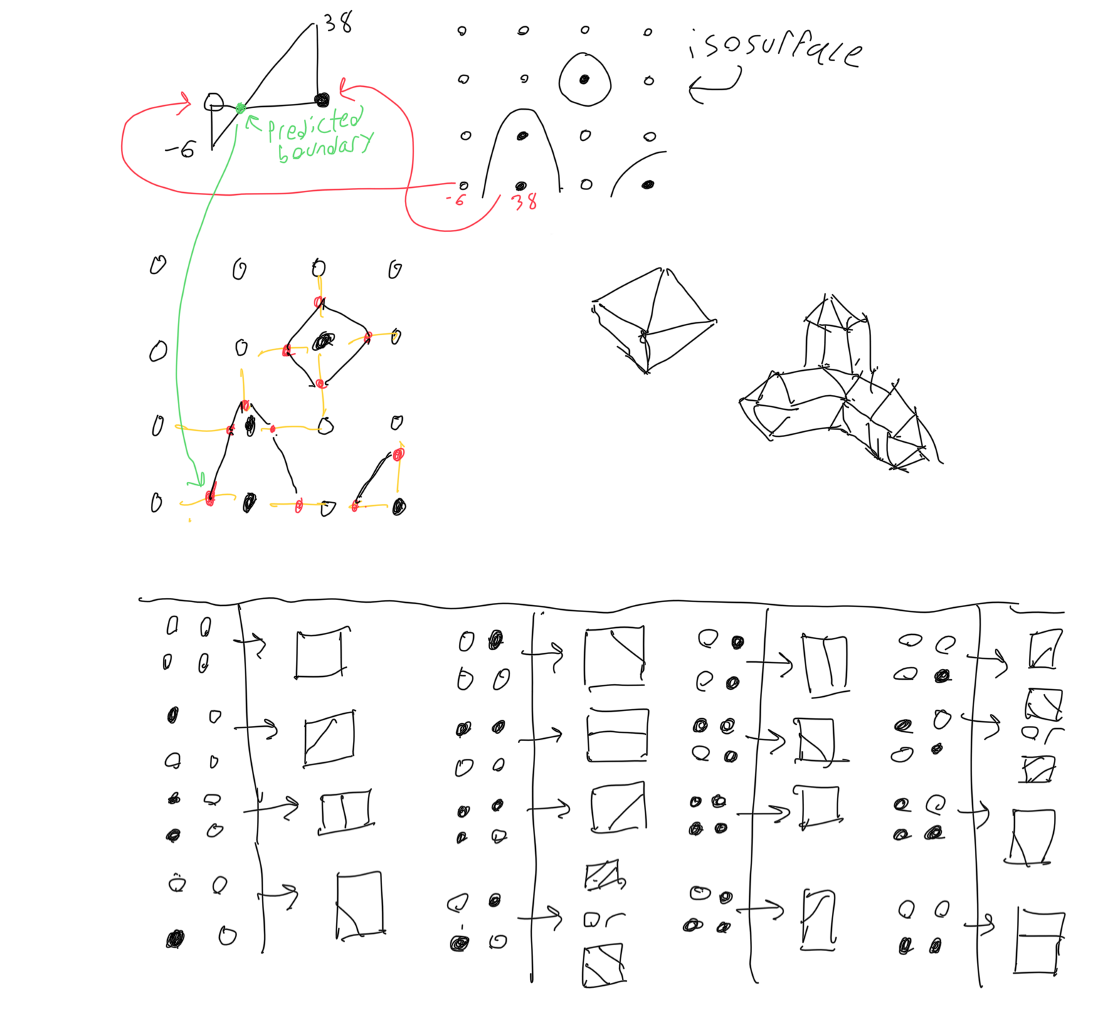
The second method, which I also experimented with, is called marching cubes. Marching cubes places all vertices along the line segments connecting the sampling points, and stitches polygons between them according to a lookup table with the opaqueness of the surrounding vertices. To use this method, the program must make an estimate at where boundary of an isosurface lies, given two points, one above zero, one below zero. This is done linearly. The figure below illustrates this in 2D with four vertices and 16 entries in the lookup table, but the concept extends to 3D where eight vertices would be considered with 256 entries in the table. Marching cubes is most commonly used in medical imaging. It produces only smooth meshes (or at least beveled meshes) This is an improvement, because the voxel boundary has another degree of freedom- vertices can be placed anywhere on the line segment between the two sampling points, allowing for ground that isn’t perfectly even.
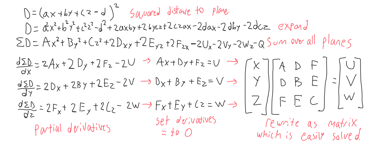
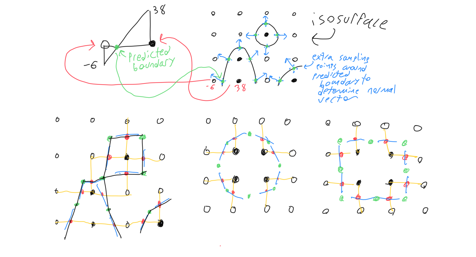
The extra degree of freedom is nice, but not perfect- The ability to have sharp corners is sacrificed, but the smoother meshes aren’t perfectly smooth, either. The last method is dual contouring: the Cadillac of isosurface extraction algorithms. The distance along the line segment between sample points must be known, same as marching cubes, but this time the vector perpendicular to the isosurface at that point much also be known. This is called hermitian data, and in addition to the linear method used to estimate the position of the boundary, six extra calls to the sampling function are used to estimate the vector perpendicular to the surface at a given point, which is called the normal. Vertices are then placed inside each box at the location that minimizes the sum of squared distances to each surrounding tangent plane. Then, stitching between vertices is done exactly like in method 1, no lookup table needed. Specifying normal information allows for both smooth and sharp meshes (and everything in between). This is how voxel games break out of their blocky, axis aligned shells.
Minimizing the squared distance to each tangent plane is a difficult process, but having a little knowledge of multi variable calculus makes things a lot easier. The figure below shows the specific math involved. The nine coefficients for each tangent plane are summed up and then turned into a 3x3 matrix which is solved to get the vertex. I’ve seen people take the pseudo inverse of a matrix with those coefficients with svd decomposition but I’ve gotten better results without that.