Proof engine solver algorithm
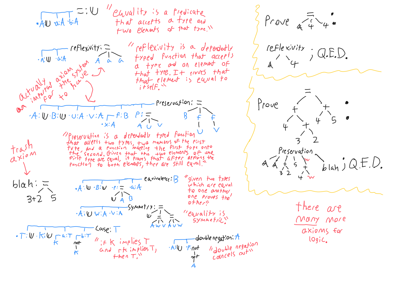
The most difficult concept to grasp in type theory is that predicates are types. The image below shows the signatures of some examples. Predicates/types may be true, false, or unprovable, but what proves a predicate to be true is if it is inhabited. In other words, if there is a valid statement whose type is predicate P, then P is proven, and the statement is its proof.
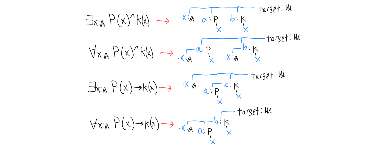
Targets are like signatures- they have a set of children which are signatures and may refer to each other. There are tricks for representing theorems as targets.
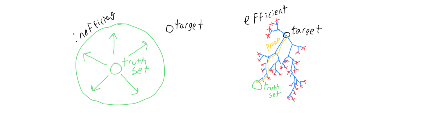
The goal of the theorem prover, then, is to find such a statement. A naive algorithm would start with its set of axioms and prove more and more predicates, expanding its ‘truth set’ until it happens to encompass the target theorem. A much more efficient approach is to work backwards instead, expanding the finite set of predicates which imply the target theorem until the set contains a statement known to be true. This approach is more focused, and has more features upon which to speed up the search. Some elements in the predicate set obsolete each other, so many of these elements can be removed during a search to keep the search space in check.
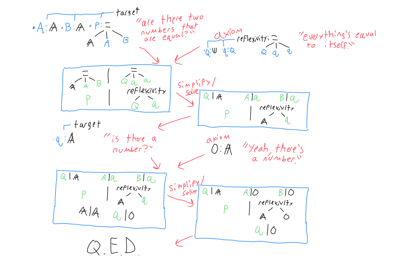
Another way to think of the problem is to set up an unknown variable whose type signature is the target predicate. The type signature may also have arguments, which allow universal quantification and preconditions. That unknown variable’s root node is either an axiom, or one of its parameters. The unknown variable can be inserted as a pair with some special rules for each possibility, with the unknown variable on the left and the possibility on the right. The first rule is that each parameter that the right hand node accepts is a new unknown variable. Each of those unknown variables’ signatures are the same as the root node’s corresponding argument, but with the left hand node’s argument signatures tacked on as extra arguments. In addition to being added as pairs, their types must be added as pairs as well. (Which is the key part of the algorithm, because it asserts that the types are judgmentally equal, ensuring that the proof is valid.) The below diagram shows one step.
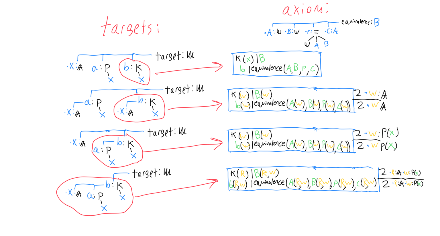
As you can see from that diagram, some of the unknowns don’t make sense to solve for. The general rule is that if an unknown’s substitution variable is referenced by another unknown’s signature, it should not be solved for. The exception is in the case of circular loops, because then there can be a situation where no unknown meets the criteria. Reference loops should usually be avoided, but as long as all axioms and targets are well-formed and consistent, they cause no problems with the algorithm. (If the input is valid, then any condition that would cause the algorithm to do an infinite substitution would sooner cause the algorithm to return ‘no solution’. And not as a cheap workaround either- there is strictly no solution in that case.) After the algorithm makes a bunch of binding objects representing attempts at solving one of the unknowns with an axiom, each binding object is simplified and split into solved forms. Some binding objects will fail, which means that axiom cannot be used to satisfy that unknown. Other binding objects will split into many solutions, meaning there is more than one way to apply that axiom in that case. Each application of an axiom may create more unknowns that need to be solved for, and it may coincidentally specify unknowns besides the one being solved for.